Quantum Primer
A practical introduction to quantum computing concepts, focused on what you need to know to solve challenges. No prior quantum experience required.
Chapters
Linear Algebra Basics
Optional — but recommended for deeper understanding
Do I need to know this to solve challenges?
No. You can solve every challenge on Qubit Forge without understanding the maths behind it. The platform tells you exactly which gates to use and what output to target. You do not need to do any calculations by hand.
However, if you want to understand why your circuits work, what a gate is actually doing to a qubit, and the real significance of the quantum algorithms you are building, this section will give you that foundation. Think of it as the difference between following a recipe and understanding why each ingredient matters.
Numbers: The Building Blocks
Before we talk about vectors or matrices, let's make sure we are on the same page about numbers. In everyday life you use whole numbers (1, 2, 3) and decimals (3.14, 0.5). In maths, a single number is often called a scalar — it just means "one number on its own."
In quantum computing, these scalars are usually decimal numbers (like 0.707) and sometimes involve the square root symbol. For example, . Do not worry about computing these by hand — the computer does it for you. You just need to recognise what the notation means when you see it.
Quick notation guide
The square root of 2 (about 1.414). The number which, multiplied by itself, gives 2.
1 divided by √2 (about 0.707). You will see this number constantly in quantum computing.
Pi (about 3.14159). The ratio of a circle's circumference to its diameter. Used for rotation angles.
Half of pi (about 1.571). Represents a quarter turn (90°).
Vectors: Lists of Numbers
A vector is simply an ordered list of numbers. You can think of it like a column in a spreadsheet. In quantum computing, we write vectors as a vertical stack of numbers inside square brackets:
A 2-element vector
This vector has two entries: the first is 1, the second is 0.
Another 2-element vector
First entry is 0, second entry is 1.
Why vectors matter for quantum computing
In quantum computing, the state of a qubit is a vector. The qubit in state is actually the vector , and the qubit in state is the vector . The two entries in the vector represent the "amount" of and in the qubit's state.
A qubit in superposition — part 0 and part 1 at the same time — is a vector where both entries are non-zero:
This is the "plus" state — an equal mix of 0 and 1. Both entries are equal (about 0.707 each), meaning there is a 50% chance of measuring either outcome. The is just a scaling factor that makes the probabilities add up to 1.
Complex Numbers: Not as Scary as They Sound
In school, you were probably told "you can't take the square root of a negative number." In maths, we invented a workaround: define a special number called where (in other words, ). A complex number is any number that combines a regular part and an part:
is the real part — a normal number you are already familiar with.
is the imaginary part — the coefficient multiplied by .
A normal number (zero imaginary part)
A purely imaginary number
A complex number with both parts
Why complex numbers matter
The entries in a qubit's state vector can be complex numbers (not just regular decimals). This is what gives quantum computing its extra power — the imaginary part creates a property called phase, which is how quantum algorithms manipulate probabilities through interference.
You do not need to do complex number arithmetic to solve challenges. You just need to know they exist and roughly what they mean when you see them.
Magnitude (Absolute Value) of Complex Numbers
When you see in quantum computing, that is asking: "what is the magnitude squared of this complex number?" The magnitude tells you how "big" the number is, ignoring its direction/phase:
Example: a regular number
So there is a 50% probability — exactly what we expect from a superposition state.
Example: a complex number
Even though this has an imaginary part, the probability is still 50%.
Key takeaway: in quantum computing, the probability of measuring a particular outcome equals the magnitude squared of its amplitude. means "square the real part, square the imaginary part, and add them together."
Matrices: Grids of Numbers That Do Things
A matrix is a rectangular grid of numbers. If a vector is a single column in a spreadsheet, a matrix is the whole table. In quantum computing, matrices are important because every quantum gate is a matrix.
The X gate (quantum NOT)
A 2×2 grid: 2 rows, 2 columns.
The Hadamard gate
Also 2×2. The keeps probabilities valid.
Matrix × Vector = Gate Applied to Qubit
When you "apply a gate to a qubit," the computer is multiplying the gate's matrix by the qubit's state vector. Here is how that works, step by step:
Example: Apply the X gate (NOT) to
Step 1: For the first entry of the result, take the first row of the matrix and do a dot product with the vector: .
Step 2: For the second entry, take the second row of the matrix and dot it with the same vector: .
Result: The output vector is which is . Applying the NOT gate to gives — exactly as expected!
Example: Apply the Hadamard gate to
The result is the state — equal superposition. Both entries are 0.707, so the probability of measuring 0 is (50%), and the probability of measuring 1 is also 50%. This is why the Hadamard gate creates superposition — it spreads the amplitude equally across both states.
Do I need to do matrix multiplication by hand?
Absolutely not. The computer and the simulator handle all of this automatically. The reason we show it here is so that when you read "the Hadamard gate creates a superposition," you can understand how it does that (by multiplying a matrix by a vector) and why the result is a 50% / 50% split.
Tensor Products: Combining Multiple Qubits
When you have more than one qubit, you need to describe the combined state of the whole system. This is where the tensor product (written as ) comes in. The tensor product combines two smaller vectors into one larger vector.
Example: Two qubits, both in state
The tensor product takes two 2-element vectors and produces a 4-element vector. The rule is straightforward: multiply the first entry of the left vector by every entry of the right vector, then do the same for the second entry:
(first entry of left vector × right vector)
(second entry of left vector × right vector)
Stack them:
This is written in shorthand as . The 4-element vector represents all four possible states of two qubits:
Both qubits are 0
First qubit 0, second qubit 1
First qubit 1, second qubit 0
Both qubits are 1
Why this matters
This is the mathematical explanation for why quantum computers are potentially powerful: qubits need a vector with entries. Just 10 qubits require a vector of 1,024 entries. 30 qubits need over a billion entries. A quantum computer handles this naturally — a classical computer has to store and manipulate all of those numbers explicitly.
For challenges: you will not need to calculate tensor products. But when a challenge says "create the state ," you now know this describes a 4-element vector where the 1st and 4th entries are non-zero (those two states both have amplitude).
Connecting the Dots: Dirac Notation
Now you know what vectors are, you can understand the notation used throughout this primer and on the platform. Quantum physicists invented a shorthand called Dirac notation (or "bra-ket notation") so they do not have to write column vectors every time:
The and symbols are just visual wrappers — they tell you "this is a quantum state vector." It is like how quotation marks tell you something is a word: "cat" is a label for the animal, and is a label for the vector .
Putting it all together
This equation, which appears at the start of Chapter 1, now makes complete sense: a qubit's state is a 2-element vector. The first entry () is how much is in the mix, and the second entry () is how much . The probability of measuring 0 is (magnitude squared, as we learnt above), and the probability of measuring 1 is .
Section Summary
What you need for challenges
- Recognise Dirac notation (, , )
- Know that qubit states are described by amplitudes
- Understand that gives a probability
- Know that gates change the state of qubits
- Accept that more qubits = exponentially larger state space
Helpful but not required
- Understanding what vectors and matrices are
- Complex numbers and the role of phase
- How matrix multiplication transforms states
- How tensor products build multi-qubit spaces
- Why unitary matrices keep probabilities valid
Qubits and States
Classical Bits vs Qubits
A classical bit is either 0 or 1. A qubit (quantum bit) can also be 0 or 1, but unlike a classical bit, it can exist in a superposition of both states simultaneously. This is the foundational concept behind quantum computing.
Superposition
When a qubit is in superposition, it has some probability of being measured as 0 and some probability of being measured as 1. These probabilities are described by complex numbers called amplitudes.
New to this notation? Read the Linear Algebra Basics section first — it explains everything from scratch.
A qubit's state can be written as:
Where and are complex amplitudes. The probability of measuring 0 is and the probability of measuring 1 is . These probabilities always sum to 1.
Need a maths refresher?
The Linear Algebra Basics section above covers vectors, complex numbers, matrices, and tensor products from scratch — no prior maths background required.
Dirac Notation
Quantum states are written using Dirac notation (also called bra-ket notation). This is the standard notation used in quantum computing and you will see it throughout challenge descriptions.
The "zero" state. A qubit that will always measure as 0. This is the default initial state of qubits.
The "one" state. A qubit that will always measure as 1.
Equal superposition: . Created by applying a Hadamard gate to . 50% chance of measuring 0 or 1.
Minus superposition: . Created by applying a Hadamard gate to . Also 50%, but with a different phase.
Multi-Qubit States
When you have multiple qubits, the state space grows exponentially. Two qubits have four possible states: , , , and . Three qubits have eight possible states, and so on. A system of qubits has basis states.
This exponential growth is the source of quantum computing's potential power. A classical computer needs numbers to describe qubits, but the qubits themselves exist in this full space naturally.
Quantum Gates
Quantum gates are operations that transform qubit states. They are the quantum equivalent of classical logic gates (AND, OR, NOT), but they work on superpositions and must be reversible (unitary).
Single-Qubit Gates
X Gate (Pauli-X)
qc.x(qubit)The quantum NOT gate. Flips to and vice versa. Often called a "bit flip."
Z Gate (Pauli-Z)
qc.z(qubit)Leaves unchanged but maps to . Introduces a "phase flip" that affects interference. Has no effect on measurement probabilities alone.
Y Gate (Pauli-Y)
qc.y(qubit)Combines the effects of X and Z (with a factor of ). Flips the state and adds a phase.
Hadamard Gate (H)
qc.h(qubit)The most important single-qubit gate. Maps to (equal superposition) and to . Applying H twice returns to the original state.
S Gate (Phase Gate)
qc.s(qubit)Adds a phase to . A "quarter turn" around the Z-axis of the Bloch sphere. .
T Gate
qc.t(qubit)Adds a phase to . A finer rotation than S. . Important for fault-tolerant quantum computing.
Rotation Gates
Rotation gates allow precise, continuous control over qubit states. They take an angle parameter and rotate the qubit around a specific axis of the Bloch sphere.
qc.rx(θ, qubit)X-axis rotation
qc.ry(θ, qubit)Y-axis rotation
qc.rz(θ, qubit)Z-axis rotation
, (up to global phase). Rotation gates generalise the Pauli gates and are essential for variational quantum circuits.
Phase and the Bloch Sphere
You have seen that a qubit's state has amplitudes. But amplitudes are complex numbers, and complex numbers carry a property called phase. Phase is the angle of the complex number in the complex plane — it does not change the probability of measuring 0 or 1, but it has a dramatic effect on how amplitudes combine during interference.
Global phase vs relative phase
Global phase
Multiplying the entire state by a number like changes nothing measurable. The states and are physically identical. You can ignore global phase.
Relative phase
A phase difference between the amplitudes of and does matter. The states and both have 50% measurement probabilities, but they behave very differently in circuits because the minus sign (a phase of ) changes how they interfere.
Why does phase matter?
Quantum algorithms work by making correct answers interfere constructively (amplitudes add up) and wrong answers interfere destructively (amplitudes cancel out). Phase controls whether amplitudes add or cancel.
The Z, S, and T gates all work purely by adjusting phase. They do not change measurement probabilities directly — their effect only shows up when combined with other gates like the Hadamard.
The Bloch Sphere
The Bloch sphere is a visual way to represent a single qubit's state as a point on the surface of a sphere. Every single-qubit pure state corresponds to exactly one point on this sphere.
The Bloch sphere. The arrow (state vector) points to the current state of the qubit. Every point on the surface is a valid single-qubit state.
North pole
Qubit is definitely 0
South pole
Qubit is definitely 1
Equator (+X)
Equal superposition (positive phase)
Equator (−X)
Equal superposition (negative phase)
How gates move the state on the sphere
X gate: 180° rotation around the X-axis. Flips the qubit from north pole to south pole (or vice versa).
Z gate: 180° rotation around the Z-axis. Flips the phase. becomes and vice versa, but and stay unchanged.
Hadamard (H): Swaps the Z-axis and X-axis. Takes (north pole) to (equator) and (south pole) to .
Rotation gates (): Rotate by any angle around their respective axis. This includes every single-qubit gate as a special case.
Do I need to memorise the Bloch sphere?
No. The Bloch sphere is a visualisation tool. It is helpful for building intuition about what gates do — especially phase gates that do not change measurement probabilities. If it helps you, use it. If not, you can solve every challenge without it.
Multi-Qubit Gates
CNOT (CX)
qc.cx(control, target)The controlled-NOT gate. Flips the target qubit if and only if the control qubit is . The most common two-qubit gate. Essential for creating entanglement.
CZ
qc.cz(control, target)Controlled-Z. Applies a Z gate to the target if the control is . Symmetric: it does not matter which qubit you call control or target.
SWAP
qc.swap(qubit1, qubit2)Exchanges the states of two qubits. Equivalent to three CNOT gates. Useful when you need to rearrange qubit positions.
Toffoli (CCX)
qc.ccx(ctrl1, ctrl2, target)Double-controlled NOT. Flips the target only when both control qubits are . The quantum equivalent of a classical AND gate.
Gate matrices
Every quantum gate is represented by a unitary matrix. For single-qubit gates, this is a 2×2 matrix. For two-qubit gates, it is 4×4. You do not need to know the matrices to solve challenges, but understanding them helps conceptualise what gates do to quantum states.
Circuits and Measurement
Building Circuits
A quantum circuit is a sequence of gates applied to qubits. Gates are applied left-to-right (in the order you write them in code). All qubits start in the state unless otherwise specified.
A circuit that creates the Bell state :
qc = QuantumCircuit(2)
qc.h(0)       # Hadamard on qubit 0 → creates superposition
qc.cx(0, 1)   # CNOT: entangles qubit 0 and qubit 1
# Result: (|00⟩ + |11⟩)/√2
Circuit Depth
Circuit depth is the number of time steps needed to execute the circuit, assuming gates on different qubits can run in parallel. It measures the critical path length, not the total gate count.
Example: Depth 2
H on qubit 0, then CNOT(0,1). Two layers of operations. The H must finish before the CNOT can use qubit 0.
Example: Depth 1
H on qubit 0 and X on qubit 1 simultaneously. These operate on different qubits, so they run in the same time step.
Measurement
Measurement collapses a qubit's superposition into a definite classical value: 0 or 1. The probability of each outcome is determined by the amplitudes of the quantum state.
Measurement is probabilistic
A qubit in the state has a 50% chance of measuring 0 and 50% chance of measuring 1. You cannot predict which outcome will occur for a single measurement.
Measurement is destructive
After measurement, the superposition is destroyed. The qubit collapses to whichever state was observed. You cannot "un-measure" a qubit.
Statistical results
By running a circuit many times (shots), you build up a probability distribution. With enough shots, the distribution converges to the true probabilities.
Measurement Notation
For a qubit in state , the Born rule gives the probability of each outcome:
After a 0 outcome the qubit collapses to ; after a 1 outcome it collapses to . In Qiskit, explicit measurement syntax looks like:
qc = QuantumCircuit(2, 2)   # 2 qubits, 2 classical bits
qc.h(0)
qc.cx(0, 1)

# Measure individual qubits into classical bits
qc.measure(0, 0)   # qubit 0 → classical bit 0
qc.measure(1, 1)   # qubit 1 → classical bit 1

# Or measure all qubits at once
qc.measure_all()
Platform note
On Qubit Forge, your circuits are evaluated using a statevector simulator, which computes exact probabilities without needing to run thousands of shots. You do not need to add measurement gates -- the platform handles this automatically.
Reading Quantum Circuits
When you solve a challenge on Qubit Forge, the results panel shows a circuit diagram of the circuit your code built. This chapter teaches you how to read those diagrams. Every image below was generated with the exact same renderer used in the challenge results, so what you see here is what you will see there.
Qubit Wires
Each horizontal line represents one qubit. Wires are labelled on the left-hand side. Every qubit starts in the state unless your code prepares it differently.
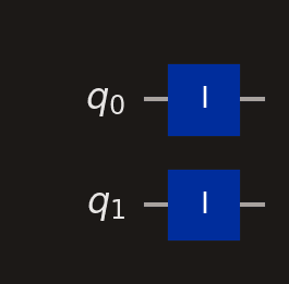
A two-qubit circuit with no gates applied. The identity (ID) gates are placeholders — they do nothing to the state.
Reading Left to Right
Time flows from left to right. The first gate on the wire is applied first. In the diagram below, the Hadamard (H) gate executes before the X gate.
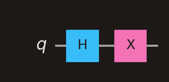
H is applied first, then X. The order matches the code: qc.h(0); qc.x(0)
Gate Symbols & Colours
Each gate type has a distinct colour so you can identify them at a glance. The colours below are the same ones used in challenge results.
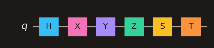
Single-qubit gates in sequence: H (sky), X (pink), Y (purple), Z (emerald), S (amber), T (orange).
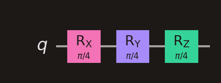
Rotation gates share colours with their Pauli counterparts: Rx (pink like X), Ry (purple like Y), Rz (emerald like Z). The angle parameter is shown inside the box.
Multi-Qubit Gate Notation
Multi-qubit gates span two or more wires. The vertical line connecting the wires shows which qubits are involved. Each gate type uses a different symbol.
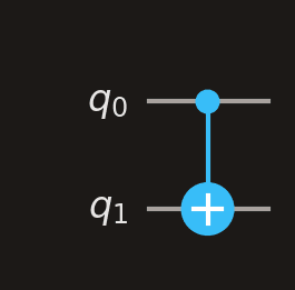
CNOT (CX)
A filled dot marks the control qubit. A circled-plus (⊕) marks the target. The target is flipped only when the control is .
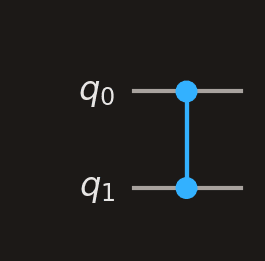
CZ
Two filled dots connected by a line. CZ is symmetric — it does not matter which qubit you call control or target. Applies a Z gate when both qubits are .
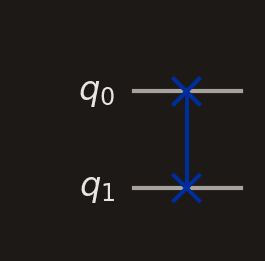
SWAP
Two × symbols connected by a line. Exchanges the states of the two qubits.
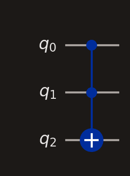
Toffoli (CCX)
Two control dots and one circled-plus target. The target is flipped only when both controls are .
Measurement
Measurement is shown as a meter symbol. A double line emerges from the measurement, representing the classical bit that stores the result. Classical bits are labelled and drawn as a separate register at the bottom of the diagram.
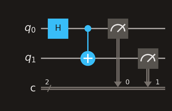
A Bell state circuit followed by measurement on both qubits. The grey meter boxes collapse the quantum state into classical bits (the double lines at the bottom).
Putting It Together
Here is a complete Bell state circuit without measurement — exactly as it would appear in your challenge results. Read it left to right: first H creates a superposition on , then CNOT entangles with .
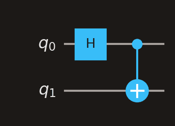
The Bell state . This is the circuit you would build for challenge #6 (CNOT gate).
Tip
On Qubit Forge you do not need to add measurement gates — the platform measures automatically. The diagrams in your results show the circuit before measurement so you can focus on the quantum operations.
Practice: trace these circuits
After submitting each challenge below, open the results panel and compare the generated diagram against the code you wrote. Check that every gate and wire matches your intent.
Single H gate on one qubit. The simplest possible diagram — one wire, one box.
Two-qubit circuit. Look for the control dot connected to the target gate.
H + two CNOTs across three qubits. Trace each column left to right and verify the qubit connections.
Entanglement
What Entanglement Is (and Isn't)
Entanglement is a correlation between qubits that has no classical equivalent. When two qubits are entangled, measuring one instantly determines the state of the other, regardless of the distance between them.
Entanglement IS
Entanglement IS NOT
- Faster-than-light communication
- Cloning or copying quantum states
- A way to send information instantly
- The same as classical correlation
Bell States
The Bell states are the four maximally entangled two-qubit states. They are the simplest examples of entanglement and appear frequently in challenges.
Entanglement as a Resource
Entanglement is not just a curiosity -- it is a computational resource. Quantum algorithms exploit entanglement to achieve speedups over classical algorithms. Key applications include:
- Quantum teleportation: transferring quantum states using entanglement and classical communication
- Superdense coding: sending two classical bits using one qubit and shared entanglement
- Quantum error correction: protecting information by encoding it across entangled qubits
- Algorithm speedups: Grover's search and Shor's factoring both rely on entanglement
Algorithms Overview
Quantum Parallelism
A quantum computer can evaluate a function on all possible inputs simultaneously by preparing a superposition of inputs. This is not the same as classical parallelism -- you cannot directly read out all results. The art of quantum algorithms is designing circuits that extract useful information from the superposition through measurement.
Interference and Amplitude Manipulation
Quantum algorithms work by manipulating amplitudes so that correct answers have higher probability and wrong answers have lower probability. This is achieved through interference:
Constructive Interference
Amplitudes add together, increasing the probability of a particular outcome. Correct answers are amplified.
Destructive Interference
Amplitudes cancel each other out, reducing the probability of a particular outcome. Wrong answers are suppressed.
Key Algorithm Families
These algorithm families appear in Master-level challenges. Understanding the high-level idea is more important than memorising implementations.
Deutsch-Jozsa
Determines whether a function is constant or balanced using a single query. The simplest demonstration of quantum speedup. Tests your understanding of oracles and interference.
Grover's Search
Searches an unsorted database in time versus classically. Uses amplitude amplification: mark the target state, then amplify its amplitude through repeated Grover iterations.
Quantum Phase Estimation (QPE)
Estimates the eigenvalue (phase) of a unitary operator. A fundamental subroutine used in many other algorithms, including Shor's algorithm for factoring.
Variational Quantum Eigensolver (VQE)
A hybrid classical-quantum algorithm for finding ground state energies. Uses parameterised circuits with rotation gates. The classical optimiser adjusts gate angles based on measurement results.
Quantum Fourier Transform (QFT)
The quantum analogue of the discrete Fourier transform. Operates exponentially faster than its classical counterpart. Core component of phase estimation and factoring algorithms.
Practical Considerations
On Qubit Forge, you are not just solving for correctness -- you are solving for efficiency. These practical techniques help you design better circuits.
Circuit Depth Management
Parallelise independent operations
If two gates act on different qubits, they can execute in the same time step. Apply them back-to-back in your code and Qiskit will optimise the depth.
Avoid unnecessary serialisation
Only create dependencies between gates when the algorithm requires it. A Hadamard on qubit 0 and an X on qubit 1 have no dependency.
Use native multi-qubit gates
A single CNOT is depth 1. Decomposing it into multiple single-qubit operations increases depth unnecessarily.
Gate Count Optimisation
Combine rotations
Two consecutive gates on the same qubit can be combined into a single with the summed angle. Three H gates = one H gate (since ).
Choose the right gate
Use the most direct gate for the job. If you need a phase flip, use Z directly rather than .
Eliminate identity operations
Applying a gate and then its inverse accomplishes nothing. , , . Remove these redundancies.
Why Constraints Matter
Qubit Forge challenges impose constraints for a reason: on real quantum hardware, every gate introduces noise (errors) and every qubit is expensive. Efficient circuits are not just an academic exercise -- they are essential for practical quantum computing.
- Fewer gates = less accumulated noise on real hardware
- Shallower circuits = less decoherence (qubits lose their quantum properties over time)
- Fewer qubits = more practical deployability on current hardware
- Constraint awareness is a core quantum engineering skill that employers value
What's Next
This primer covers the core concepts used in Qubit Forge challenges. For deeper learning, explore the external resources on the main Resources page, or start solving challenges to apply what you have learned.